The boost in computing power and easy availability tools since 2012 have seen a rise of formation and usage of Deep Learning Models. While many are still busy limiting themselves into building new Models or improving accuracy, they are unaware of the lying attacks which seem to deteriorate or hamper there model.

Here we are going to discuss the Adversarial attack, it carries a technique of misclassifying the input image of a Deep Learning model. Subtle perturbations to input image which is far to be perceived normally can largely differ or fool the model to predict incorrect outputs. Perturbations are noise that is added to a clean image to make it an adversarial example.

The adversary performs either White Box or Black Box attacks. Former attack expects an adversary to know the architecture, inputs, outputs of the model. While later limits adversary to know only inputs and outputs of the model.

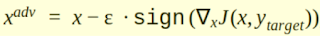
Considering Targeted Fast Gradient Sign Method to show the attack:

We have taken the squeeze net model to serve the purpose,

import torchvision.models as models

squeezenet = models.squeezenet1_1(pretrained=True, progress=True)

Above is the target model on which we will be applying the attack.

Now we need to download the dataset for the model, the dataset downloaded are having images on which we'll add perturbations.

imageNet_dataset = datasets.ImageNet('../data', split='val', download=True,
            transform=transforms.Compose([transforms.ToTensor(), normalize]))

Epsilons considered to run the test ranges are:

epsilons = [0, .05, .1, .15, .2, .25, .3]

We have kept 0 in the list of epsilons because it represents model performance on the original test set. Higher epsilons are taken to have higher perturbations.

At this instance we have both model and dataset ready, let's train the model:


    for data, target in test_loader:

        data.requires_grad = True
        output = model(data)
        init_pred = output.max(1, keepdim=True)[1] 
        if init_pred.item() != target.item():
            continue

        loss = F.nll_loss(output, target)
        model.zero_grad()
        loss.backward()
        data_grad = data.grad.data

TFGSM states to have gradient step computed in direction of the negative gradient

def tfgsm_attack(image, epsilon, data_grad):
    sign_data_grad = data_grad.sign()
    perturbed_image = image - epsilon*sign_data_grad
    perturbed_image = torch.clamp(perturbed_image, 0, 1)

    return perturbed_image


Attacking the model :

        perturbed_data = tfgsm_attack(data, epsilon, data_grad)

Re-classify the perturbed image


        output = model(perturbed_data)

Check for the final prediction and determine the accuracy of attack

    final_pred = output.max(1, keepdim=True)[1]
    final_acc = correct/float(len(test_loader))

    print("Epsilon: {}\tTest Accuracy = {} / {} = {}".format(epsilon, correct, len(test_loader), final_acc))

Here correct is the counter when the final prediction is equal to the actual target.

Testing for all values of epsilons:

for e in epsilons:
    acc, ex = test(model, test_loader, eps)

Findings:

Plotting the accuracy with respect to epsilon values:

What's going wrong to have these attacks?

The trainability of the model to the data might be the issue when we consider a large input set and perturbation above. We might imagine the small amount of perturbation in input image pixel can be enough to change the neural network I/O.
The other way of saying the neural network flawed i.e behave differently for new data can be a prevention of this attack. Trainability and robustness have added the pain, paving the way to such attacks.

References:

1.Threat of Adversarial Attacks on Deep Learning in Computer Vision: A Survey by Navdeep Akhtar and Ajmal Mian.

2.Breaking-neural-networks-with-adversarial-attacks blog by Anant Jain

3. Code Snippets from Nathan Inkawhich